Teaching

In this page, some animations, pictures, and derivations are given to facilitate Toby's teaching.

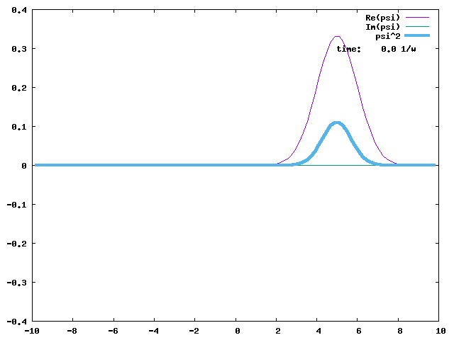
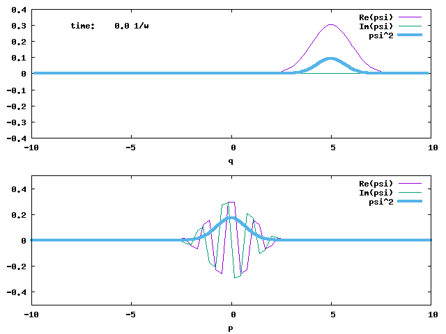
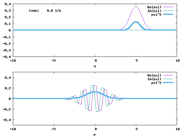
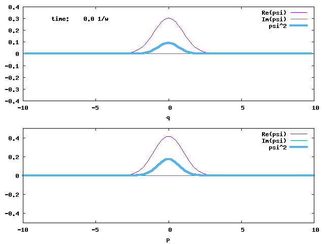
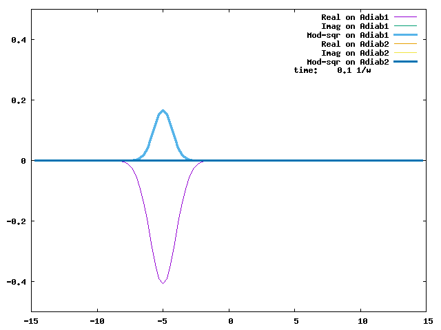
1. Evolution of a 1-D displaced Harmonic Oscillator ground state. This is a coherent state initially centred at q = 5. The angular frequency ω is 1 for the displaced ground state and the harmonic potential that propagates the state. The width of the state is conserved. The evolution time is in the unit of 1/ω. The angular frequency of the wave packet oscillation is ω.

The most generic displacement operator is defined and can be rewritten as:

It translates a state by √2α_r along the reduced position q and by √2α_i along the reduced momentum p, simultaneously. The initial coherent state above is obtained by acting the D(5/√2) operator on the H.O. ground state. Since αa^† - α*a is an antihermitian operator, D(α) is a unitary operator, and D(α)^† = D(α)^-1 = D(-α).

The simultaneous displacement in position and momentum can be decoupled to a position displacement first, and then a momentum displacement. Given two operators A and B, e^A+B = e^Ae^Be^{-[A, B]/2}, if [[A, B], A] = [[A, B], B] = 0.

The decoupling of the position and momentum displacement is accomplished. It must come with a phase factor, whose phase is negative half of the product of the two displacement magnitudes, -√2α_r√2α_i/2. Acting this form of the displacement operator on the H.O. ground state in the position representation:

The coherent state is an eigenstate of the annihilation operator, with the eigenvalue α:

Since now we call the displaced state |α〉: D(α)|0〉= |α〉; a|α〉=α|α〉.

The weights of the H.O. eigenstates in a coherent state follow a Poisson distribution, with a |α|² mean. S = |α|² is called the Huang-Rhys factor. Sω (or Sħω) gives the average energy of |α〉on top of the ground state energy ½ω, i.e., the average excitation energy of |α〉. S hence has the meaning of the average vibron (or phonon, in solid state) number. Sω also gives the reorganization energy, since it is the energy emitted when the excited H.O. fully relaxes to its ground state. In classical mechanics, this relaxation corresponds to the reorganization of the H.O. from its non-equilibrium position to its equilibrium position.

Using the same trick of e^A+B = e^Ae^Be^{-[A, B]/2}, if [[A, B], A] = [[A, B], B] = 0, we can write D(α) = e^-|α|2/2 e^αa†e^α*a. 〈0|α〉=〈0|D(α)|α〉= e^-|α|2/2〈0|e^αa†e^α*a|0〉= e^-|α|2/2〈0|e^αa†|0〉= e^-|α|2/2. Then we have

After determining the coherent state as an expansion in the H.O. eigenstates, it is straightforward to determine its evolution under the H.O. Hamiltonian:

α(t) = αe^iwt/2, the time-dependent displacement parameter (or eigenvalue of the annihilation operator). So, in the position representation, |〈q|0〉|² maintains its Gaussian shape, with with an evolving complex-valued displacement √2α(t): √2α_r(t) on q and √2α_i(t) on p.

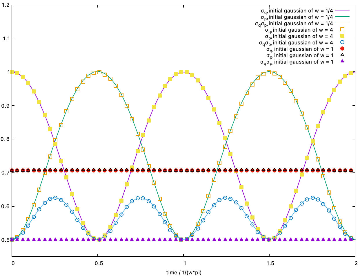
Writing the initial α as α = re^iφ, then α(t) = re^-i(wt-φ), α_r(t) = r cos(wt - φ), and α_i(t) = -r sin(wt - φ). The position and momentum displacements oscillate like a classical H.O. The shape-preserved oscillation is demonstrated by the animation above. The π/2-off shape-preserved oscillation in the momentum space is seen below, in the comparison with the oscillation in the position space.

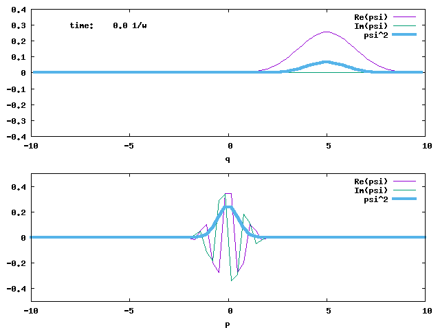
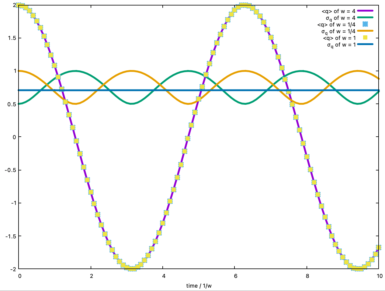
2. The same as 1, but the displaced H.O. ground state is prepared for the H.O. Hamiltonian with ω = 4. The width of the Gaussian is broadened when it comes to q=0, the bottom of the ω = 1 H.O. potential. The broadening in the q-wave packet corresponds to the sharpening of the p-wave packet.

3. The same as 1, but the displaced H.O. ground state is prepared for the H.O. Hamiltonian with ω = 1/4. The width of the Gaussian is sharpened when it comes to q=0, the bottom of the ω = 1 H.O. potential. In 2 and 3, the widths oscillate with the gaussian wave packet, but in opposite directions. The two states are squeezed states.

The oscillations of centres (<q>) and widths (σ_q) of the coherent and squeezed states in 1-3 are shown below.

If we only squeeze the states but without the displacements, the non-displaced squeezed states evolve as below.

Initial gaussian with w = 4:

Initial gaussian with w = 1/4:

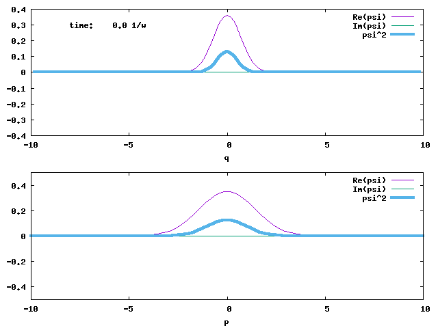
Initial gaussian with w = 1:

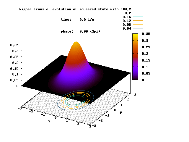
Shown below is the Wigner transform of the evolving squeezed state with the initial squeeze parameter ξ = 0.2.

Shown below is the Wigner transform of the evolving displaced squeezed state with the initial squeeze parameter ξ = 0.5 and the initial displacement parameter α = 5.0.

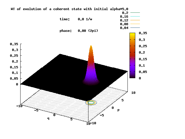
Shown below is the Wigner transform of the evolving non-squeezed coherent state with the initial displacement parameter α = 5.0.

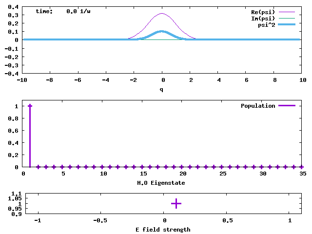
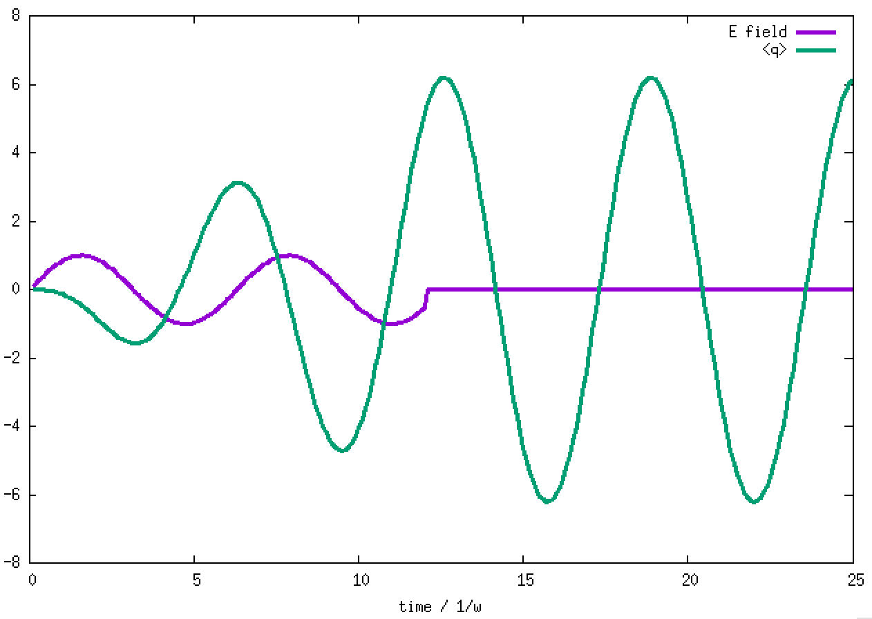
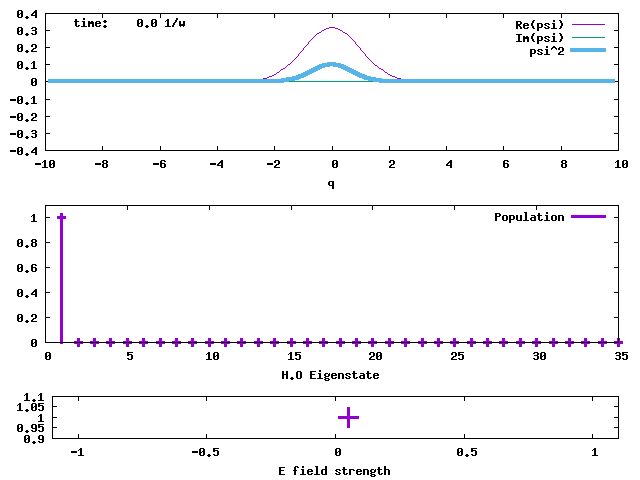
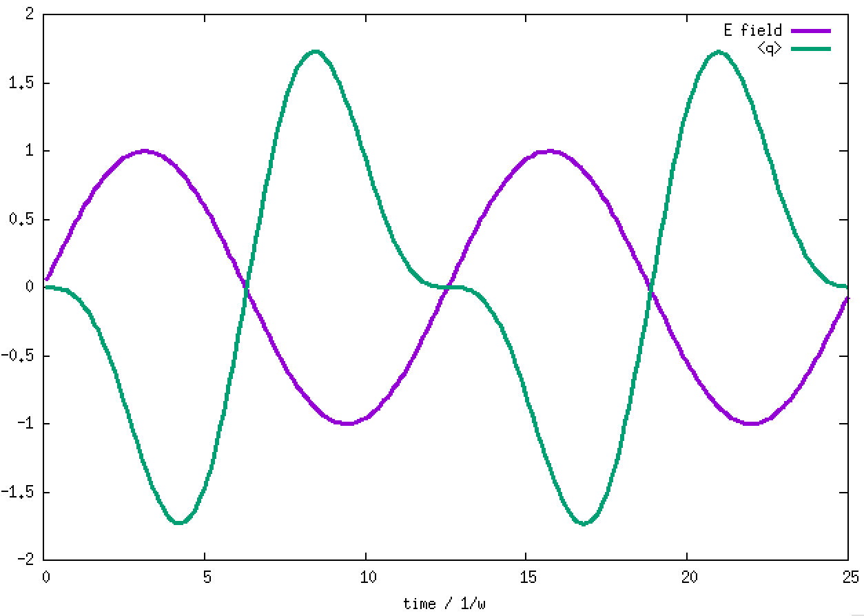
4. Taking the H.O. ground state as the initial state, an electric field taking the form of E*sin(ωt) is applied to the state. The field is sketched in the bottom panel. The transition dipole moment between adjacent H.O. eigenstates is taken to be sqrt(1/2) and E is taken to be 1. The oscillating field in resonance with the H.O. pumps the stationary ground state to an oscillating coherent state, maintaining its Gaussian shape and width. When the <q> average value is greater than 5 at time = 12/ω, the field is turned off. The coherent state then keeps oscillating without changing the amplitude. The oscillating electric field acts like a "displacement operator" to displace the Gaussian from the stationary minimum position to an oscillating wave packet. The evolutions of the populations of the H.O. eigenstates in this pumped coherent state are shown in the lower panel. The populations follow the Poisson distribution, P_n = e^-d2 (d²)ⁿ/n!. sqrt(2)d is the displacement of the Gaussian wave packet from the minimum of the H.O. potential. Clearly, in the end, the lowest-lying states are not populated, against the normal situation of Boltzmann distribution (Bose-Einstein distribution as well). What will result from such a population inversion? If we don't turn off the oscillating electric field, what will happen to the wave packet and the populations? The answer should be obvious.

If the time's arrow is reversed, the oscillating wave packet will create an oscillating electric field, i.e., emitting an electromagnetic radiation, and the populations will be back to the normal situation of only the lowest states being populated.

The oscillation of the E-field and <q> are shown in the graph below.

The evolutions of both the q- and p-wave packets are shown below.

When the angular frequency of the oscillating E field is set to be 2, the results are shown below. There is no population inversion. We push a "swing" with a twice of its intrinsic frequency, the swing doesn't go high.

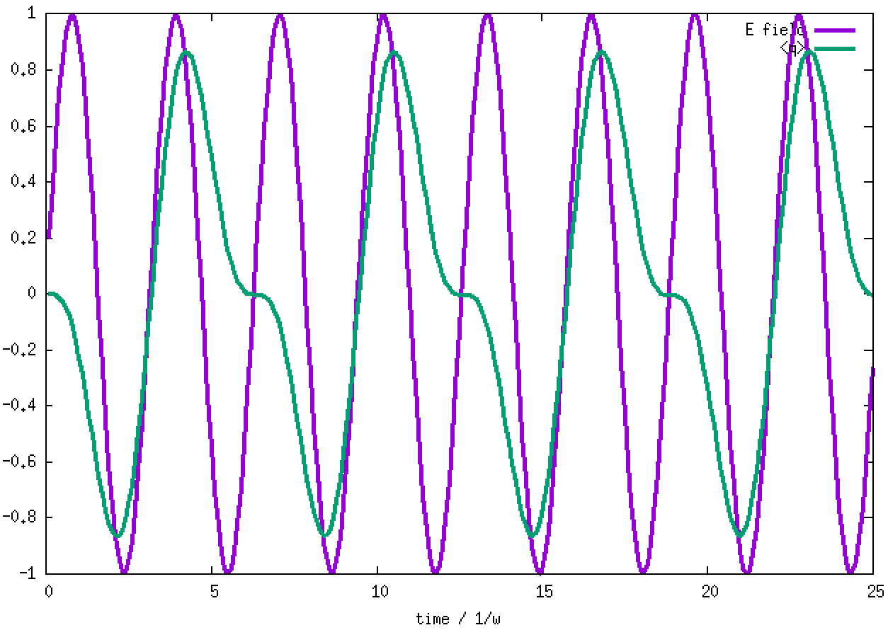
When the angular frequency of the oscillating E field is set to be 0.5, the results are shown below. There is also no population inversion. We push a "swing" with a half of its intrinsic frequency, the swing oscillates with the push frequency, instead of its intrinsic frequency.

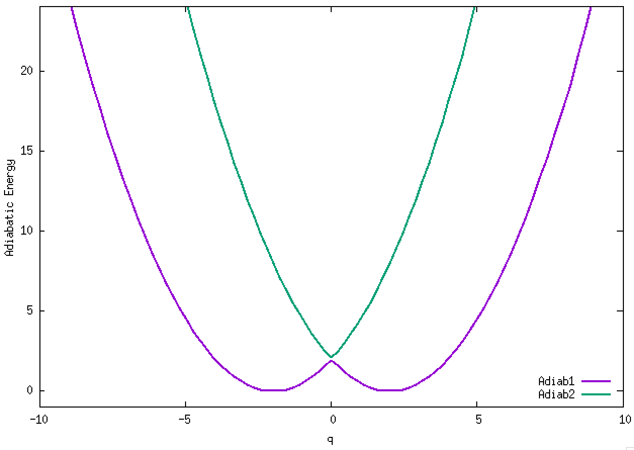
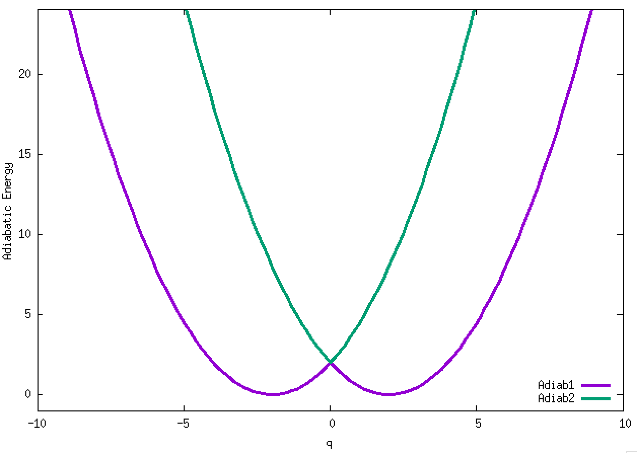
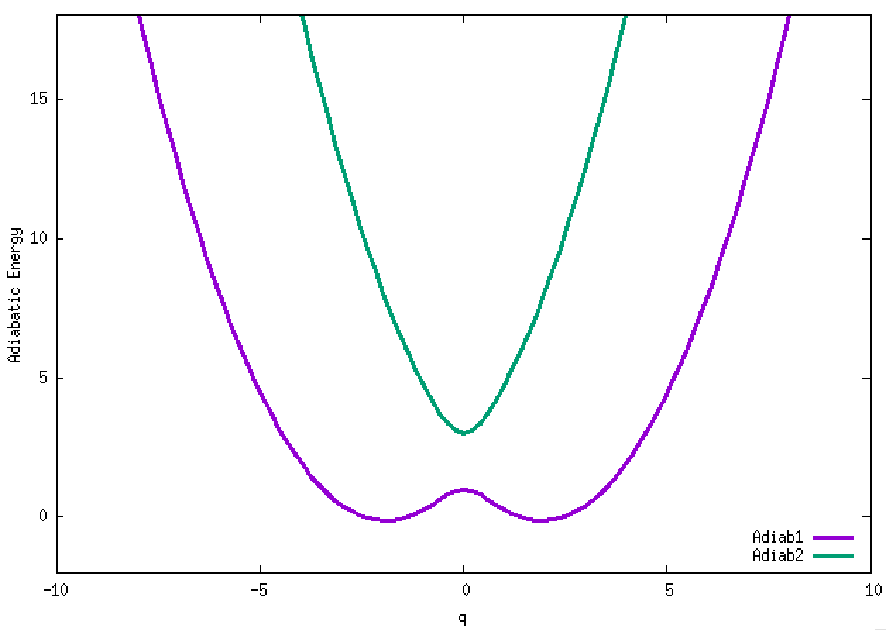
4. Adiabatic energies of two diabats with symmetrically-displaced harmonic potential ½(q ± 2)² and a weak constant coupling of -0.1. The two diabats are called left and right diabats according to their minima. This is a typical strong non-adiabatic coupling case. We will examine several non-adiabatic dynamics for this vibronic Hamiltonian.

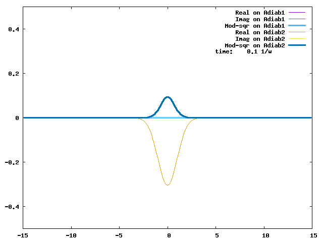
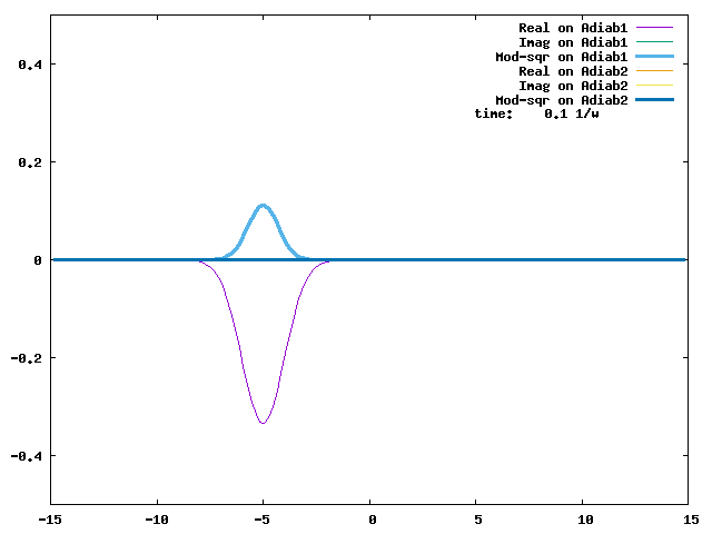
4.1. A Gaussian wave packet whose width is consistent with the diabatic potentials is initially placed at q=-5 and at the 2nd adiabatic state (i.e., on the green adiabatic curve). While it mainly oscillates on the potential energy curve of the right diabat, the weak -0.1 coupling brings a little bit of the wave packet to the left diabat whenever it crosses the avoided crossing at q=0. In the picture of the adiabats, the wave packet remains on the right diabat corresponds to a non-adiabatic transition at q=0. We can see the color change (change of adiabats) of the wave packet whenever it passes through q=0. The weak -0.1 coupling leads to a large F₁₂ non-adiabatic coupling at q=0, which facilitates transition from one adiabat to the other. At the same time, the weak coupling also leads to large positive -½G₁₁ and -½G₂₂ diagonal Born-Oppenheimer correction (DBOC). These large "potentials" of the adiabats prevent the wave packet from remaining on the same adiabat while transmitting between the two sides of the avoided crossing. G₁₁ = G₂₂ = -(F₁₂)²: the prevention of remaining on the same adiabat comes with the facilitation of transitioning to the other adiabat. It is hence illogical to keep DBOC in adiabatic potentials while ignoring the non-adiabatic coupling F_IJ.

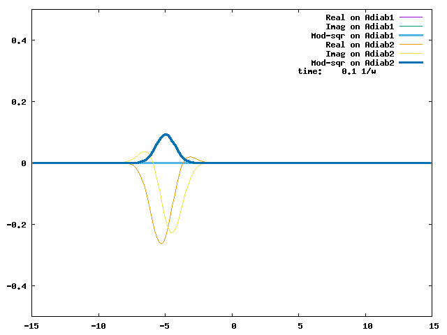
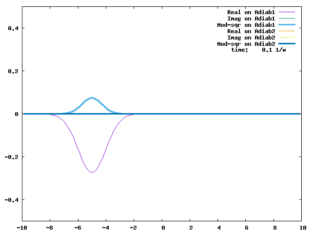
In the animation below, everything is the same except that the initial wave packet is placed at the ground state Adiab1. Compared to the case above, there is a bit more probability for the wave packet to remain on the ground state (see the purple and green curves, the cyan curve is not as obvious) when it passes through the avoided crossing at q=0. The less efficient Adiab1-to-Adiab2 transition compared to the efficient Adiab2-to-Adiab1 transition above is attributed to the smaller momentum of the wave packet when it reaches q=0. The smaller momentum is attributed to the lower potential difference between q=-5 and q=0 on the Adiab1 potential energy curve.

4.2. The setting of the evolution below is almost identical to the setting in 4.1, except that the diabatic coupling is 0 across the whole range of q. Therefore, the two adiabats sharply exchange their diabatic characters at q=0, and the avoided crossing above has become a crossing in the adiabatic energy curves below. The wave packet strictly evolves on the right diabat. Since the right diabat changes from one adiabat to another at q=0, the wave packet undergoes a complete non-adiabatic transition between the two adiabats at q=0 (|F₁₂| = ∞). There is no remaining on the same adiabat (-½G₁₁ = -½G₂₂ = ∞). The color change of the wave packet as it crosses q=0 is sharp, and there is strictly no overlap between the cyan and indigo parts of the wave packet. The vibronic wave function is continuous and well-behaved. The apparent discontinuity of the wave packet in the adiabatic representation is cancelled by the discontinuity of the adiabats.

4.3. The setting of the evolution below is identical to the situation in 4.2, except that the initial wave packet is centred at q=0, the crossing point. The wave packet propagates far away immediately. This anomalous behaviour must arise from anomalies in the initial vibronic state. Adiabat 2 is discontinuous at q=0. Placing a continuous vibrational wave packet on this discontinuous adiabat results in a discontinuous vibronic initial state. If we transform the initial vibronic state to the diabatic representation, the wave packet on the left and right diabats sharply decay to 0 at q=0. This discontinuity in the vibrational wave packet gives some components of infinite momentum to the wave function, which propagates far away immediately after t=0. As the matter of fact, this discontinuous initial vibronic state cannot be prepared.

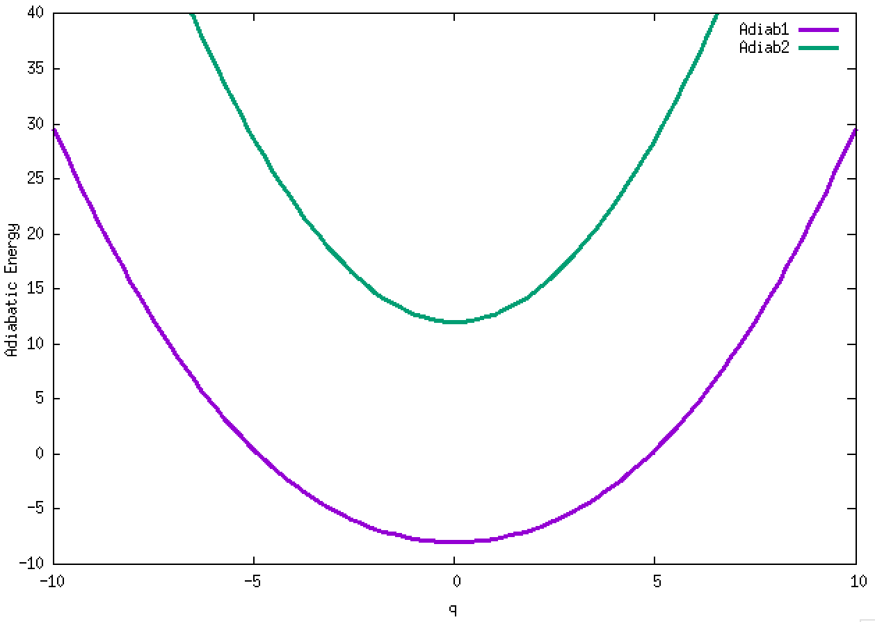
4.4. Now we consider the typical adiabatic case. The setting is identical to 4.1, except that the constant coupling is set to the -10 large magnitude. The adiabatic energies are shown below.

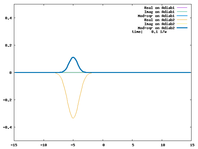
The evolution of the wave packet which is initially placed at q=-5 and on Adiab2 is shown below. There is essentially no transition to Adiab1. The tiny little bit of wave packet on Adiab1 (the purple and green curves) that shows up when the wave packet on Adiab2 samples the bottom of E2 transits back to Adiab2 when the wave packet leaves the bottom.

The evolution of the wave packet when it is initially placed at Adiab1 is shown below. Similarly, the wave packet essentially evolves only on Adiab1.

Adiabatic approximation works well for this large potential coupling case. Large potential coupling between diabats means weak non-adiabatic coupling between adiabats. In the other way around, weak potential coupling between diabats means strong non-adiabatic coupling between adiabats.

 

4.5. For the intermediate situation of coupling being -1, the ground state potential energy curve shows a smooth barrier, as shown below.

The evolution of the initial wave packet placed at q=-5 and on Adiab2 is shown below. The Adiab2-to-Adiab1 transition is still significant, with the minimum gap = 2. The wave packet on Adiab1 has more kinetic energy to samples more area, and hence visits the q=0 area less often than the wave packet on Adiab2. Therefore, the overall trend we see is from Adiab2 to Adiab1.

When the initial wave packet is placed on Adiab1, with all the other settings being identical, the evolution of the wave packet is shown below. The Adiab1-to-Adiab2 upward transition is less significant than the Adiab2-to-Adiab1 downward transition above. The wave packet mostly stays on Adiab1.

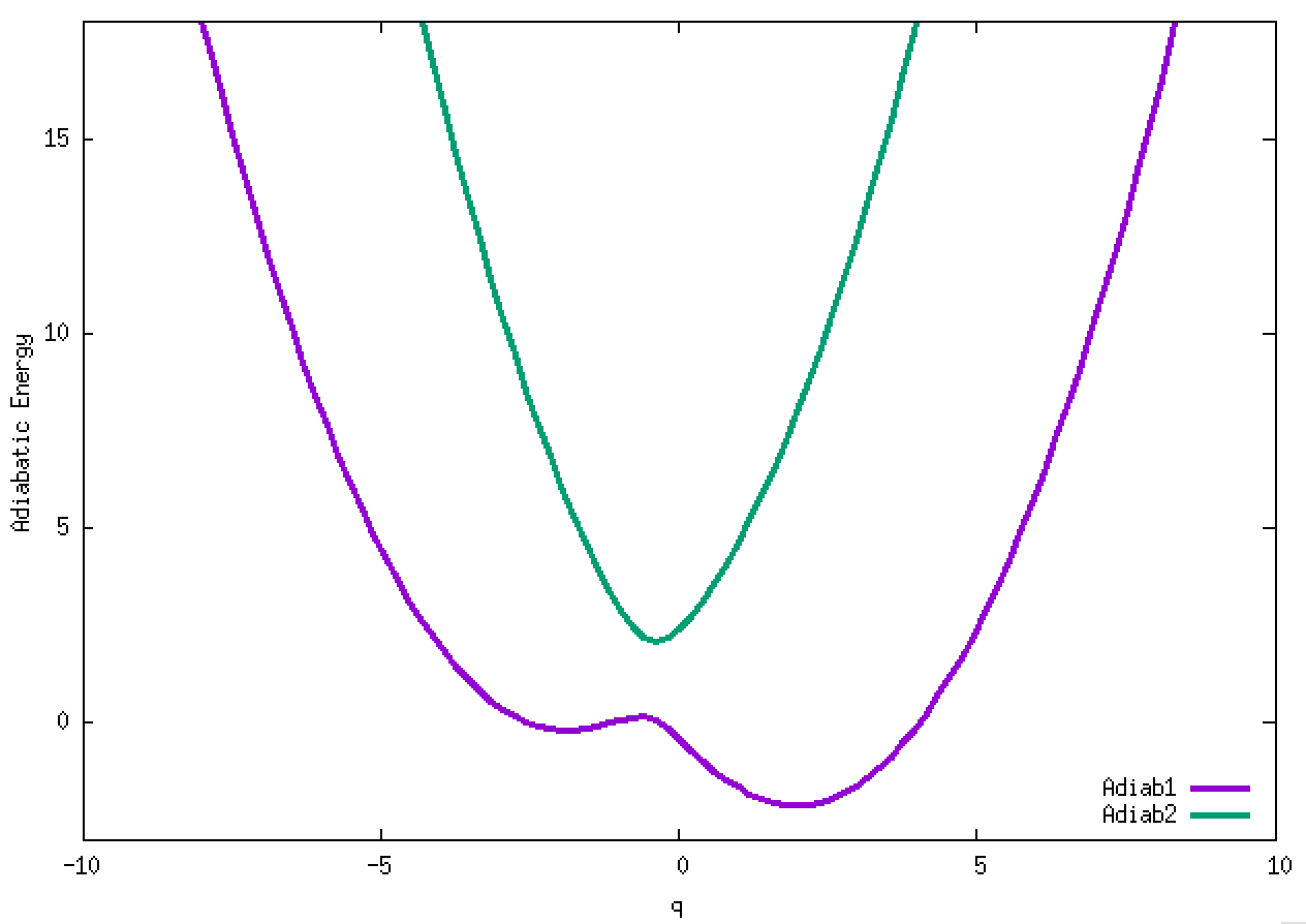
4.6. We take the vibronic Hamiltonian in 4.5, but now shift down the right diabat's energy by 2. The resultant asymmetric adiabatic potential energy curves are shown below.

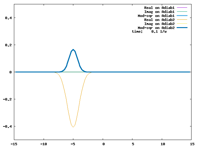
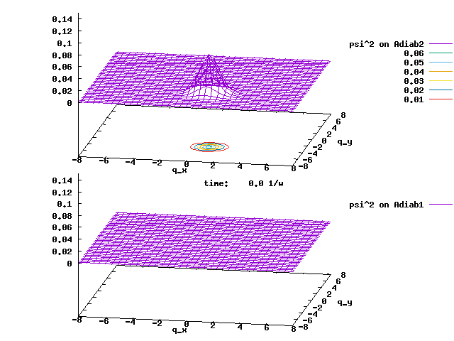
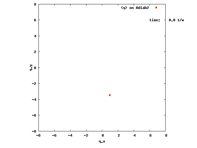
The evolution of a wave packet initially placed at q=-5 and on Adiab2 is shown below. If we stop the watch at t = 4.5/w, we can see that the Adiab2-to-Adiab1 transition is almost complete. This time marks the moment that the wave packet on Adiab2 has sampled the avoided crossing twice and spawned two wave packets on Adiab1 on the two sides of the avoided crossing, and the spawned wave packets on Adiab1 have not had a chance to sample the avoided crossing yet. With efficient energy dissipation, the wave packets are likely to stay on Adiab1.

Shown below are the evolutions of the populations on the two adiabats. At the short time, the population conversion is one way, from the initial high energy Adiab2 to the low energy Adiab1. However, as the population on Adiab1 accumulates, the backward transition to Adiab1 is seen. Eventually, the populations of the two states evolve to close to equivalence, with a small fluctuation. This is the typical situation when there is no dissipation of energy, so that the population in Adiab1 is not thermodynamically favoured.

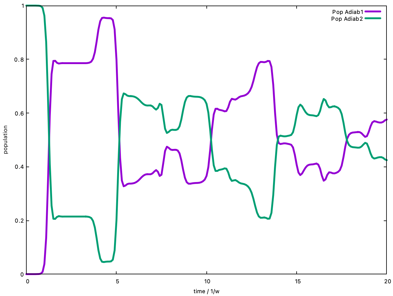
When the initial wave packet is placed on Adiab1 while all the other settings are the same, the evolution is shown below. Compared to the case above, the upward transition is much more difficult.

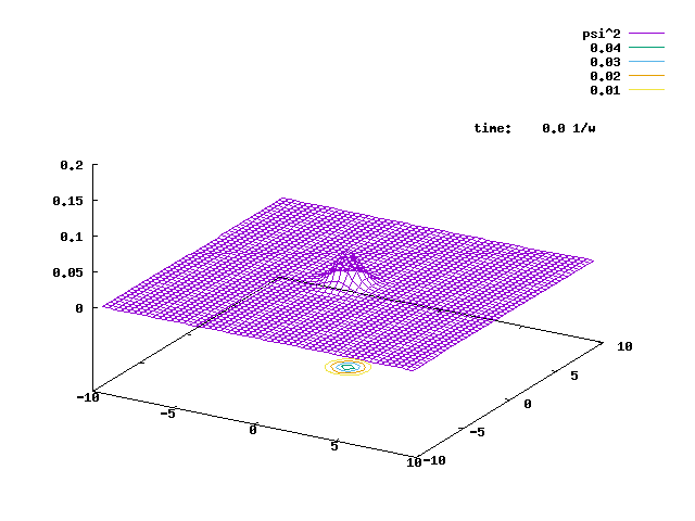
5. In this part, we go over some 2D H.O. states.

5.1. The animation below is a cylindrically symmetric 2D H.O. ground state under a rotating electric field with the same angular velocity as the H.O., E(t) = E(q_x sin(wt) + q_y cos(wt)). The rotating field pushes the 2D Gaussian to become a rotating coherent state, with the same angular frequency w, and larger and larger displacement. The E-field is turned off at t = 10.6/w, when the displacement from the origin is larger than 5. The radius of the rotation is then fixed.

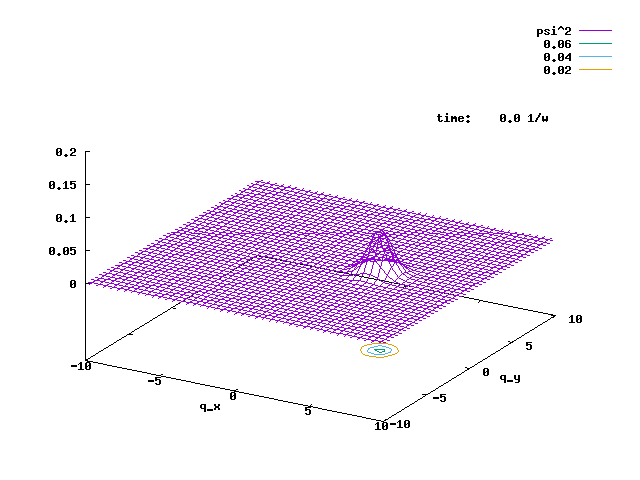
5.2. A 2-D H.O. ground state is displaced to (5,0) as the initial state to prepare the initial state. The state then evolves under the 2-D. H.O. Hamiltonian, but with an extra bilinear term Vq_xq_y, with the coupling strength V=0.1. The animation of the evolution is shown below.

6. In this part, we present some animations and figures of vibronic problems with two electronic states and two vibrational modes.

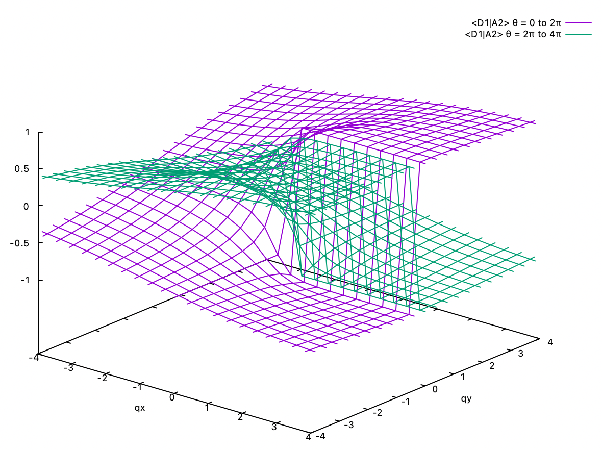
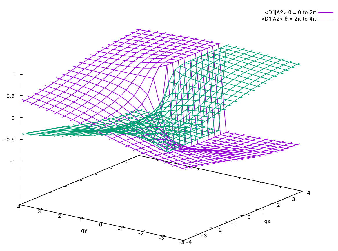
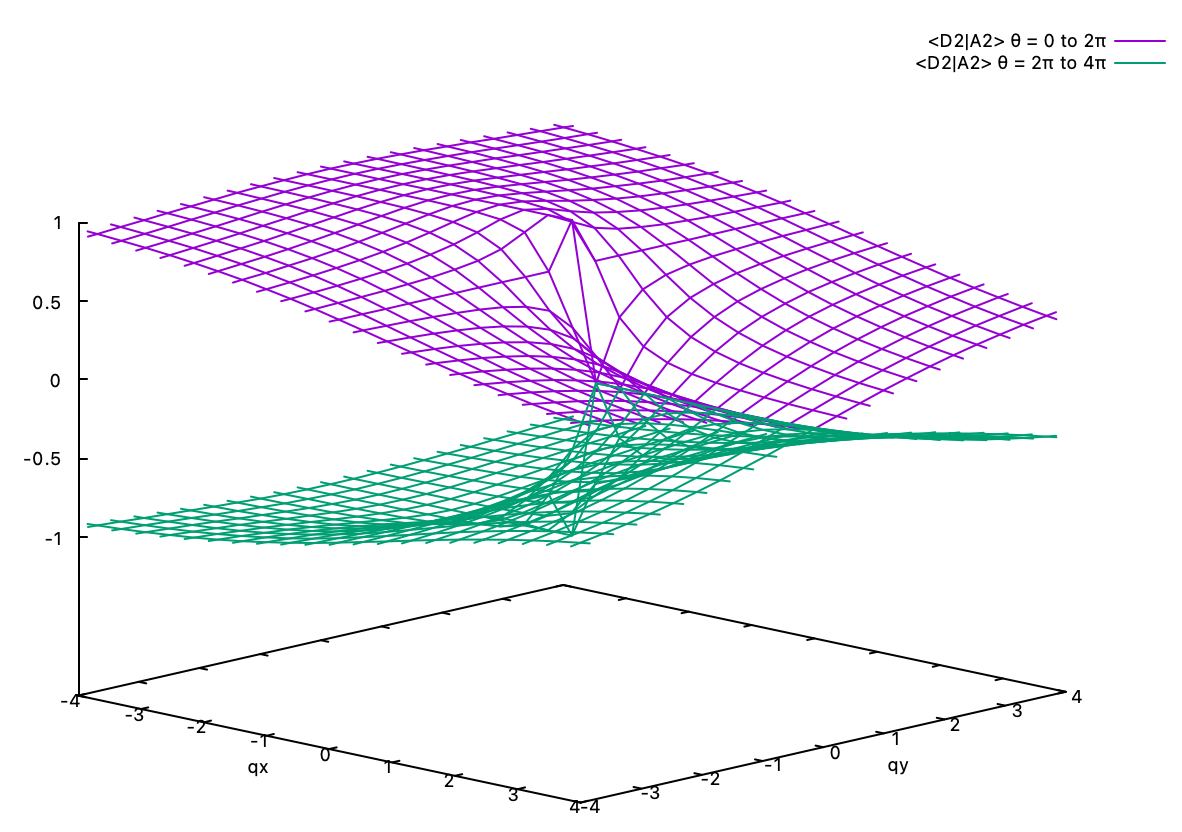
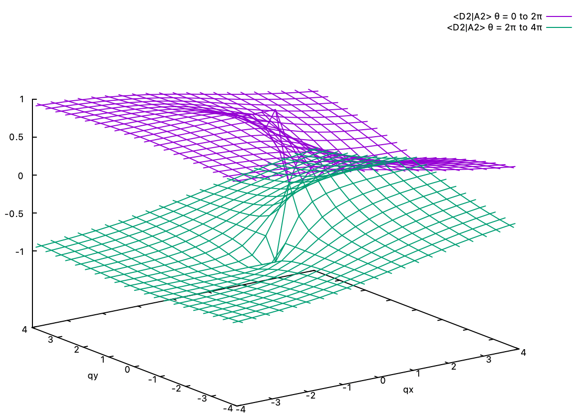
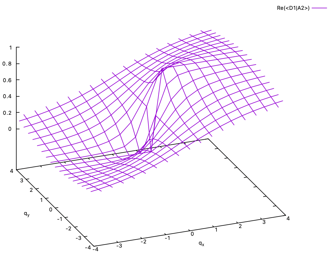
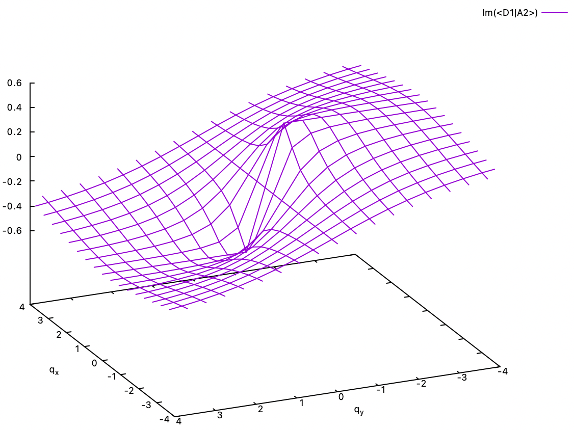
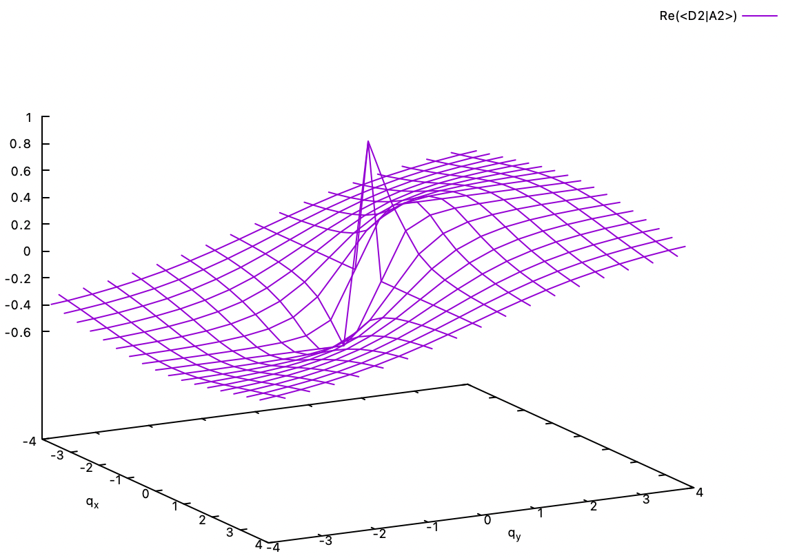
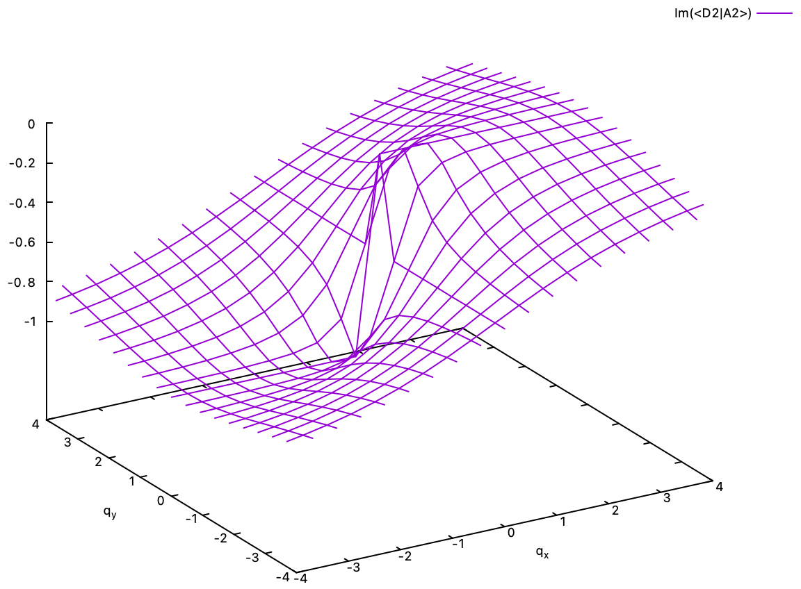
6.1. Geometric phase. Shown below are the <D1|A2> and <D2|A2> eigenvector coefficients of the two diabats D1 and D2 in the A2 adiabat in the linear E x e Jahn-Teller problem. The coefficients of the A1 adiabat are related to these coefficients by orthogonality. Two different perspectives are given for each coefficient. Clearly, if we start at the point in the positive qx axis, e.g., (2,0), and go one round in the counterclockwise direction around the origin and back to (2,0), the coefficients change their signs. The -1 is the geometric phase gained by the adiabat for travelling around the conical intersection at (0,0). If we continue another round, i.e., φ = 0 to 2π, then followed by φ = 2π to 4π, the coefficients regain their original value.

6.2. Multiplication of phase to make single-valued adiabats. The gain of the -1 phase on looping around the conical intersection can be counterposed by multiplying e^-iθ/2 phase to the adiabats. But now the adiabats are complex-valued. The real and imaginary parts of the phase-corrected <D1|A2> and <D2|A2> eigenvector coefficients are shown below. Except for the discontinuity at the conical intersection, the coefficients, i.e., the adiabats, are continuous and single-valued. The two degenerate adiabats at the conical intersection can be freely mixed and are still eigenstates of the electronic Hamiltonian. It is in principle impossible to determine them there.

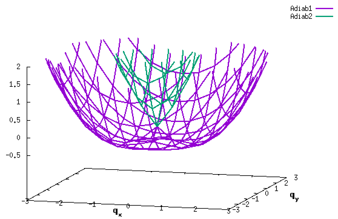
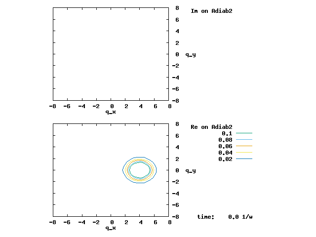
6.3. Propagation of wave packet through the E x e linear JT conical intersection. We set the diabatic electronic Hamiltonian to be H₁₁ = ½(q_x² + q_y²) + q_x, H₂₂ = ½(q_x² + q_y²) - q_x, H₁₂ = H₂₁ = q_y. The resultant adiabatic PESs are shown below. The linear JT model gives cylindrically symmetric PESs and hence a cylindrically symmetric conical intersection. The eigenvector information is shown in 6.2, i.e., an e^-iθ/2 phase has been multiplied to the adiabats to make them single-valued.

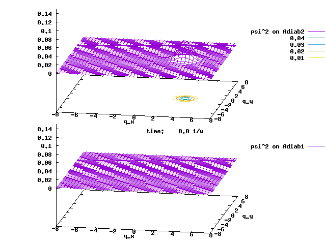
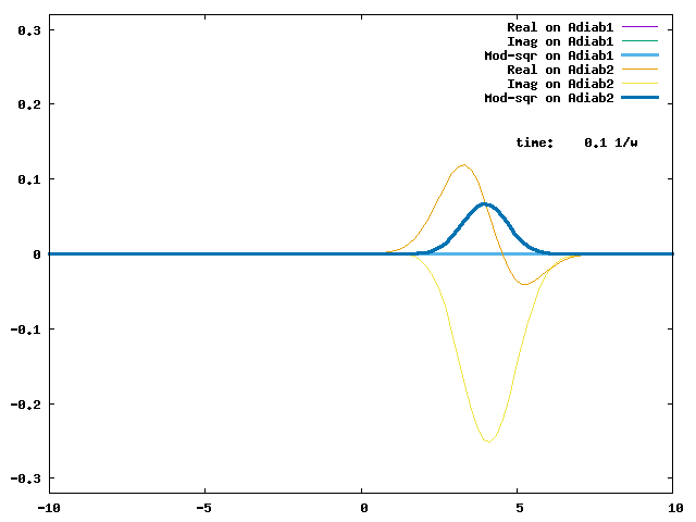
An initial wave packet as a 2D H.O. coherent state is placed at (4,0) and on Adiab2. The evolution of this wave packet by the linear JT vibronic Hamiltonian is shown below. The two panels are for the wave packet on the two adiabats, respectively. Although the wave packet is smooth almost everywhere, it spikes (i.e., it is discontinuous) at the conical intersection of (0,0). This is because the phase-corrected adiabats, despite their continuity almost everywhere, they are and must be discontinuous at the conical intersection, as explained above.

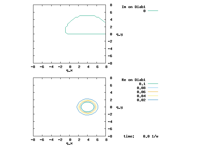
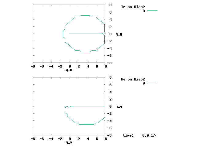
Actually, plotted above are the modular squares of wave packets and therefore, the same animations are obtained regardless of whether we use the complex-valued phase-corrected single-valued adiabats or the real-valued double-valued adiabats. The discontinuity of the real-valued adiabats is reflected by the animations below for the contour of the wave packet, instead of its modular square.

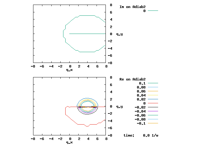
The discontinuity of the adiabats at the +q_x axis (φ = 0) is clearly shown by the real and imaginary parts of the wave packet on Adiab2, which are forced to always have opposite values on the two sides of the +q_x axis. The analogues of the phase-corrected complex-valued single-valued adiabats are shown below. The discontinuity at the +q_x axis is gone. The node on the -q_x axis of the wave packet on Adiab2 is a true node. It appears in both single- and double-valued Adiab2. It is not induced by geometric phase. Instead, it is induced by -½G₂₂ = ∞ at the conical intersection, which prevents any wave packet tunnelling on Adiab2 from the +q_x axis side to the the -q_x axis side. Similarly, the -½G₁₁ = ∞ at the intersection prevents any tunnelling on Adiab1 from the -q_x axis side to the the +q_x axis side. Therefore, there is a node in the single-valued Adiab1 wave packet in the +q_x axis.

The wave packet contour plots on the diabats are given below. No discontinuity appears, even at the conical intersection, as it should be. The linear coupling along q_y in H₁₂ guarantees that when the wave packets on Diab1 and Diab2 have different parities along the q_y axis. The odd q_y-parity of the Diab2 wave packet corresponds to the +q_x axis node of the Adiab1 wave packet and the -q_x axis node of the Adiab2 wave packet.

Shown below are the wave packets of the phase-corrected single-valued adiabats along on the q_x axis. Up to t = 5/w, the evolution largely resembles the situation in 4.2. This is as expected, since the cross section of the 2D adiabatic PESs in 6.3 looks similar to the 1D adiabatic PECs in 4.2. However, as time further gone by, the wave packet diffuse along the perpendicular q_y direction and the resemblance does not last longer. Please note that a corse q_x grid (the 2D grid is the square of the 1D grid) is used and the wave packets look jagged. We smoothened them using cubic spline and consequently, the wave packet on Adiab2 (Adiab1) does not sharply decay to 0 when it approaches q_x = 0 from the positive (negative) side. And the modular squares of the wave packet have a little negative bump around q_x = 0. But all these imperfections shall not impair our understanding of the wave packet evolution.

6.4. A rotating wave packet over the conical intersection. We prepare a 2-D H.O. rotating coherent wave packet as in 5.2, with a 4.0 distance from the origin. The wave packet is placed at Adiab2 as the initial state, which is then propagated using the linear E x e JT Hamiltonian. The resultant evolution is shown below. The wave packet mostly remains its rotation on Adiab2, with some smearing along the angular direction. This is normal since the adiabatic PES is no more harmonic. The rotation keeps the wave packet away from the conical intersection due to the centrifugal force, despite the down-hill Adiab2 PES to the intersection. Consequently, there is negligible transition to Adiab1.

Shown below is the evolution of the average position of the wave packet on Adiab2. It is mostly rotating. The apparent inward spiral motion is attributed to the smearing along the angular direction, instead of the genuine radial motion towards the conical intersection.

6.5. A question. If we apply a steady electric field to raise Diab1's (lower Diab2's) energy by δ and make them non-degenerate at (0,0), could we avoid the problem of geometric phase? The answer is no. Given the shift, the electronic Hamiltonian in the diabatic representation reads: H₁₁ = ½(q_x² + q_y²) + q_x + δ, H₂₂ = ½(q_x² + q_y²) - q_x -δ, H₁₂ = H₂₁ = q_y. The degeneracy point, i.e., the conical intersection, is shifted from (0,0) to (-δ,0). If we loop around (-δ,0), the real-valued adiabats will obtain the -1 phase. Now, let's consider a loop. For simplicity, let it be a circular loop, with the path of (1,0) → (0,1) → (0,-1) → (-1,0) → (1,0). In the original setting of δ = 0, this loop encloses the conical intersection, and the real-valued adiabats gain the -1 phase. This is still the case if |δ| < 1. But if |δ| > 1, then the path does not enclose the conical intersection, and the real-valued adiabats do not gain the -1 phase. In this sense, if |δ| is large enough, it can shift the conical intersection far enough, so that there is no geometric phase effect. The splitting δ can also come from chemical interaction (bonding or antibonding), and it can appear in the diagonal H₁₁ and H₂₂ or the off-diagonal H₁₂. Any such a real-valued "field", electric or chemical, cannot remove the degeneracy. However, an imaginary field in the off-diagonal element can. See below.

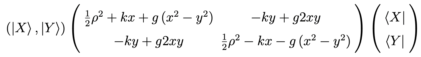
6.6. Degeneracy lifted by a magnetic interaction. The E x e linear JT vibronic Hamiltonian matrix with a magnetic interaction in two real-valued diabats (|X〉,|Y〉) representation reads:

.

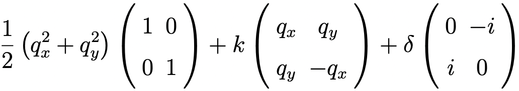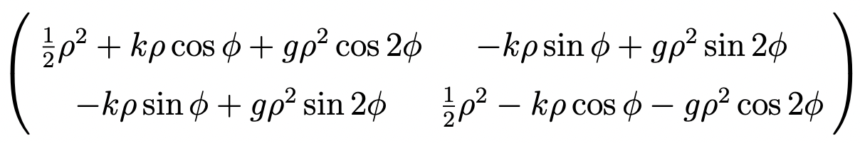
The elastic curvature has been set as the energy unit. k indicates the linear vibronic coupling strength and leads to the regular cylindrically symmetric conical intersection shown above. Without losing arbitrariness, we set k > 0. We can always change the sign(s) of |X〉and/or |Y〉to make k > 0. The third term gives a magnetic interaction between |X〉 and |Y〉, with δ indicating the interaction strength. The magnetic interaction can arise from an intrinsic field (e.g., spin-orbit coupling) or an external field. In the regular E x e JT problem, δ = 0, and (q_x,q_y) = (0,0) gives the conical intersection. When δ ≠ 0, there is no any (q_x,q_y) point to make give degenerate eigenvalues, i.e., the conical intersection is completely removed.

To analyze the eigenvalues and eigenvectors of the Hamiltonian matrix, we only focus on the second and third non-diagonal matrices. Transforming the diabats to the complex-valued diabats: |±〉 = √1/2(|X〉± i |Y〉), the non-diagonal Hermitian matrix becomes

,

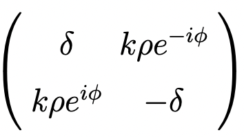where (ρ,φ) are polar coordinates of (q_x,q_y). For the situation of δ/k > 0, the eigenvectors (i.e., adiabats) are

,

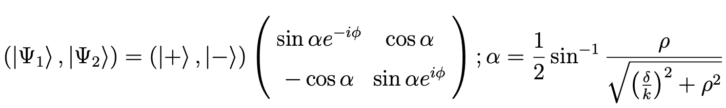for δ/k < 0, the eigenvectors are

,

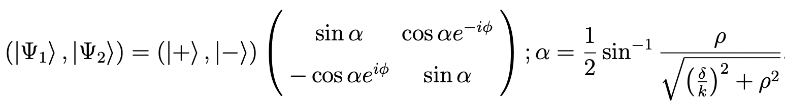and the eigenvalues are always

,

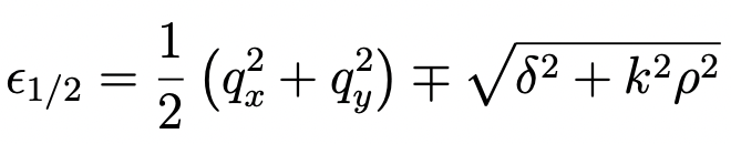regardless of the sign of δ/k. Please note that if k < 0, then the two columns of eigenvectors are swapped, while the two eigenvalues are the same. The two different forms of eigenvectors are to guarantee are connected by phase multiplications of e^±iφ. The phase-multiplication guarantees continuity of adiabats at (0,0). Please also note the different ranges of α: (1) when δ/k > 0, α ∈ [0,π/4); (2) when δ/k < 0, α ∈ (π/4,π/2]; when δ/k = 0, α = π/4.

The adiabatic energies have the smallest gap at (0,0), where only the magnetic interaction splits the two levels, while anywhere else the vibronic interaction also contributes to the splitting. The adiabats are single-valued and continuous everywhere, including at the original conical intersection (0,0). At the δ→0 limit, the adiabats become

,

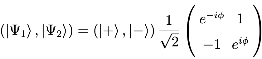which are single-valued anywhere but discontinuous (ill-determined) at (0,0), where φ is ill-determined. Then we regain the picture of the phase-corrected single-valued adiabats in the regular E x e JT problem without the magnetic interaction. The e^±iφ factors indicate that when transforming the wave packets on the |±〉diabats to the wave packets on the |Ψ_1,2〉adiabats, the diabatic wave packets main gain different vibrational angular momenta differing by the unit of ±1.

7. Geometric phase in the E x e problem.

For an E x e problem in C3v symmetry, the vibronic Hamiltonian reads

,

where k and g stand for linear and quadratic vibronic coupling constants. In polar coordinates, the diabatic Hamiltonian matrix reads

.

Any 2 x 2 real symmetric matrix eigenvalue problem can be reduced to the problem of the following matrix,

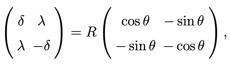
whose eigensolutions are

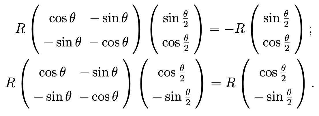
The transformation matrix between the diabats and adiabats is a rotational matrix of the angle θ/2. θ/2 is hence called the adiabat-diabat-transformation angle (ADT angle). The non-adiabatic coupling vector between the two adiabats takes the form of

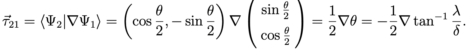
According to the gradient theorem,

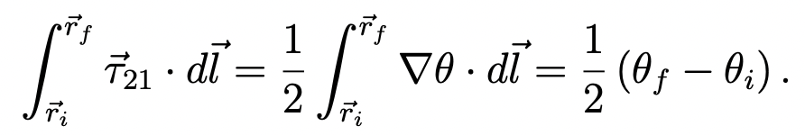
This is true if θ is differentiable along the path. θ is non-differentiable when δ=λ=0, i.e., at a degenerate point. So, if a path passes one or more degenerate points, the integral above is ill-defined. This is because the τ vector is infinite at degenerate point.